This page gives a quick introduction to linear algebra with a dedicated focus on the vector and matrix operations used in relation with Deep Learning.
Vectors
Vectors are typically introduced as representations of quantities that have direction and magnitude. For example, the velocity of a car is defined by its speed and the direction in which the car moves. This could be represented by a vector whose direction, \(\theta\), is the same as that of the car, and whose length is proportional to the speed of the car. An example of such a vector is illustrated in the figure below.
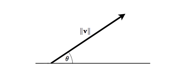 Figure 1: A vector
The above figure also lends itself well to the introduction of some notation. In the following we'll denote vectors in bold face letters, e.g. \(\mathbf{v}\), while the magnitude of a vector \(\mathbf{v}\) will be denoted by \(\left\lVert\mathbf{v}\right\rVert\). \(\theta\) is the angle between the vector and some reference direction.
Vectors are also used to specify location and displacement in a mathematical space. An example is given in figure 2 where the vector \(\mathbf{v}\) represents a displacement in the plane (shown as a bold black arrow) by \(v_1\) in the first axis and \(v_2\) in the second, i.e. \(\mathbf{v}\) can be seen as directed from the chosen origin to a point on the Cartesian plane with coordinates \((v_1, v_2)\).
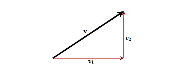 Figure 2: Vector representing a displacement in 2-dimensional space
Formally a vector is defined as an ordered set of \(n\) numbers that is usually written as a vertical array, surrounded by square brackets: $$\begin{equation} \label{eq:vector_definition} \mathbf{v} = \begin{bmatrix} v_1 \\ v_2 \\ \vdots \\ v_n \end{bmatrix} \end{equation}$$ This object is called a column vector while the values in the array are called the elements of the vector. The size (also referred to as the order, dimension or length) of the vector is the number of elements it contains. The vector above, for example, is of size \(n\) and is called an \(n\)-vector.
A horizontal array containing \(n\) numbers is called a row vector, e.g. $$\begin{equation} \label{eq:row_vector_definition} \mathbf{u} = \begin{bmatrix} u_1 & u_2 & \cdots & u_n \end{bmatrix} \end{equation}$$ If the term vector is used without being qualified further, it is understood to be a column vector as defined by \eqref{eq:vector_definition}.
Vector addition and scalar multiplication
If \(\mathbf{u}\) and \(\mathbf{v}\) are \(n\)-dimensional vectors, their sum is obtained by adding the corresponding elements of the two vectors $$\begin{equation} \label{eq:vector_addition} \mathbf{u} + \mathbf{v} = \begin{bmatrix} u_1 + v_1 \\ u_2 + v_2 \\ \vdots \\ u_n + v_n \end{bmatrix} \end{equation}$$ Geometrically vector addition can be visualized in two dimensions as simply appending one vector to the end of another. Note that \(\mathbf{u} + \mathbf{v} = \mathbf{v} + \mathbf{u}\).
Multiplying a vector \(\mathbf{v}\) by a number (i.e a scalar) \(k\) is defined as multiplying each element of the vector by \(k\) $$\begin{equation} \label{eq:vector_scalar_multiplication} k \mathbf{v} = \begin{bmatrix} k v_1 \\ k v_2 \\ \vdots \\ k v_n \end{bmatrix} \end{equation}$$ Scalar multiplication can be visualized geometrically as changing the length of the vector. If the scalar is positive then the direction of the resulting vector is not changed; if the scalar is negative the direction of the vector is reversed. Say for example we multiply a vector by \(k=-2\), then the result is a vector of twice the length (i.e. the vector has been scaled by a factor defined by the scalar), pointing in the opposite direction of the vector we started out with.
Vector subtraction can be defined in terms of vector addition and scalar multiplication $$\begin{equation} \label{eq:vector_subtraction} \mathbf{u} - \mathbf{v} = \mathbf{u} + (-1) \mathbf{v} = \begin{bmatrix} u_1 - v_1 \\ u_2 - v_2 \\ \vdots \\ u_n - v_n \end{bmatrix} \end{equation}$$ i.e. \(\mathbf{u} - \mathbf{v}\) is the addition of \(\mathbf{u}\) and a reversed copy of \(\mathbf{v}\).
Vector Transposition
Generally speaking, transposition converts row vectors into column vectors and vice versa. A given vector and its transpose form both contains the same elements, in the same order - only the "orientation" of the vector is different.
The transpose of a vector \(\mathbf{v}\) is denoted \(\mathbf{v}^\top\). Consequently the transpose of the column vector defined in \eqref{eq:vector_definition} is the row vector: $$\begin{equation} \label{eq:transpose_vector} \mathbf{v^\top} = \begin{bmatrix} v_1 & v_2 & \cdots & v_n \end{bmatrix} \end{equation}$$ while the transpose of the row vector, \(\mathbf{u}\), given by \eqref{eq:row_vector_definition} is the column vector: $$\begin{equation} \label{eq:transpose_row_vector} \mathbf{u^\top} = \begin{bmatrix} u_1 \\ u_2 \\ \vdots \\ u_n \end{bmatrix} \end{equation}$$ If we transpose a vector twice, we get back the original vector, i.e. $$\begin{equation} \label{eq:double_vector_transpose} \mathbf{(v^\top)^\top} = \mathbf{v} \end{equation}$$
Example
As an example, the transpose of \(\mathbf{v} = \begin{bmatrix} 1 \\ -2 \\ 3 \end{bmatrix}\) is \(\mathbf{v^\top} = \begin{bmatrix} 1 & -2 & 3 \end{bmatrix}\) and it's seen that transposing \(\mathbf{v^\top}\) gives us back \(\mathbf{v}\).
Inner product
The inner product, also referred to as the dot product of two column
vectors \(\mathbf{u}\) and \(\mathbf{v}\), of same order \(n\), is the scalar function:
\(\sum\) (Greek capital sigma) denotes
summation.
$$\begin{equation}
\label{eq:inner_product}
\mathbf{u} \cdot \mathbf{v} = \sum\limits_{i=1}^n u_i v_i = u_1 v_1 + u_2 v_2 + \cdots + u_n v_n
\end{equation}$$
In other words: the dot product of two column vectors is the sum of the pairwise products
of the elements of the two vectors.
Combined with the discussion on vector transposition we see that the inner product can be written using the following notation: $$\begin{equation} \label{eq:inner_product_transpose_notation} \mathbf{u} \cdot \mathbf{v} = \mathbf{u}^\top \mathbf{v} = \mathbf{v}^\top \mathbf{u} \end{equation}$$
Example
The dot product of of the two 3-vectors \(\mathbf{u} = \begin{bmatrix} 1 \\ -2 \\ 3 \end{bmatrix}\) and \(\mathbf{v} = \begin{bmatrix} 7 \\ -2 \\ -4 \end{bmatrix}\) is $$\begin{align} \mathbf{u} \cdot \mathbf{v} &= \mathbf{u}^\top \mathbf{v} \notag \\ &= \begin{bmatrix} 1 & -2 & 3 \end{bmatrix} \begin{bmatrix} 7 \\ -2 \\ -4 \end{bmatrix} \notag \\ &= 1\times7 + (-2)\times(-2) + 3\times(-4) \notag \\ &= 7 + 4 -12 \notag \\ &= -1 \notag \end{align}$$
Geometric definition of the vector dot product
In Euclidean space a vector is an object that possesses both a direction and a magnitude. Such a vector, \(\mathbf{v}\), is typically pictured as an arrow whose length represents the magnitude, \(\left\lVert\mathbf{v}\right\rVert\), of the vector. The direction of the vector is given by the direction in which the arrow points.
Suppose two vectors \(\mathbf{u}\) and \(\mathbf{v}\) are separated by an angle \(\theta\). The geometric definition of their inner product is defined as $$\begin{equation} \label{eq:inner_product_geometric_definition} \mathbf{u} \cdot \mathbf{v} = \left\lVert\mathbf{u}\right\rVert \left\lVert\mathbf{v}\right\rVert \cos(\theta) \end{equation}$$ where \(\left\lVert\mathbf{u}\right\rVert\) and \(\left\lVert\mathbf{v}\right\rVert\) are the magnitudes of \(\mathbf{u}\) and \(\mathbf{v}\) respectively.
In other words, the dot product of two vectors are defined geometrically as the size of the scalar projection of one of the vectors onto the other, multiplied with the size of the other vector (the one that is projected onto), as illustrated in figure 3.
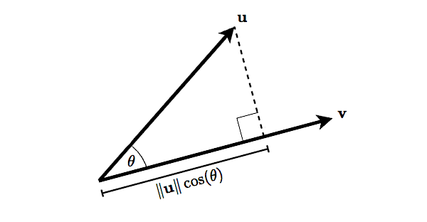 Figure 3: Scalar projection of one vector onto another
Intuitively \eqref{eq:inner_product_geometric_definition} says something about how "well aligned" two vectors are. If they are orthogonal, then \(\cos(\theta)\) is \(0\) and consequently their inner product is also \(0\). If the vectors are contradirectional - i.e. pointing in opposite directions - \(\cos(\theta)\) assumes the value \(-1\). At the other extreme, \(\cos(\theta)\) assumes the value \(1\) for codirectional vectors, i.e. vectors pointing in the same direction.
As a given vector is obviously codirectional with respect to itself, then \eqref{eq:inner_product_geometric_definition}
implies that the inner product of a vector \(\mathbf{v}\) with itself is
$$\begin{equation}
\label{eq:inner_product_of_vector_with_itself}
\mathbf{v} \cdot \mathbf{v} = \left\lVert\mathbf{v}\right\rVert ^2
\end{equation}$$
Which right away gives us the Euclidean length of \(\mathbf{v}\) as
Note that the Pythagorean theorem applied to the vector in
figure 2 gives the same result.
$$\begin{equation}
\label{eq:euclidean_length_of_vector}
\left\lVert\mathbf{v}\right\rVert = \sqrt{\mathbf{v} \cdot \mathbf{v}}
\end{equation}$$
The Euclidean length is just one way of measuring the "magnitude" of a vector, though.
So in the next section we'll have a closer look at the general concept of the
vector norm
Vector Norm
A mathematical norm is a generalization of the general concept of length or size,
i.e. a norm is a function that assigns a positive magnitude or length to each
vector in a vector space (except for the zero vector that's assigned a magnitude
of \(0\)). Formally we define a vector norm as a function
\(\left\lVert \cdot \right\rVert \colon \mathbb{R}^{n} \to \mathbb{R}\)
that has the following properties
\(\left\lvert \alpha \right\rvert\) denotes the absolute value of \(\alpha\).
For any \(\alpha \in \mathbb{R}\) the absolute value of \(\alpha\) is defined as
\(\left\lvert \alpha \right\rvert = \begin{cases} \alpha \text{, if } \alpha \ge 0 \\
-\alpha \text{, if } \alpha \lt 0
\end{cases} \)
e.g. \(\left\lvert 42 \right\rvert = 42\) and \(\left\lvert -42 \right\rvert = 42\).
Alternatively the absolute value of \(\alpha\) can be defined as
\(\left\lvert \alpha \right\rvert = \sqrt{\alpha ^2}\)
- \(\left\lVert \mathbf{v} \right\rVert \ge 0\) for any vector \(\mathbf{v} \in \mathbb{R}^{n}\), and \(\left\lVert \mathbf{v} \right\rVert = 0\) if and only if \(\mathbf{v} = 0\)
- \(\left\lVert \alpha \mathbf{v} \right\rVert = \left\lvert \alpha \right\rvert \left\lVert \mathbf{v} \right\rVert\) for any vector \(\mathbf{v} \in \mathbb{R}^{n}\) and any scalar \(\alpha \in \mathbb{R}\)
- \(\left\lVert \mathbf{u} + \mathbf{v} \right\rVert \le \left\lVert \mathbf{u} \right\rVert + \left\lVert \mathbf{v} \right\rVert\) for any vectors \(\mathbf{u}, \mathbf{v} \in \mathbb{R}^{n}\)
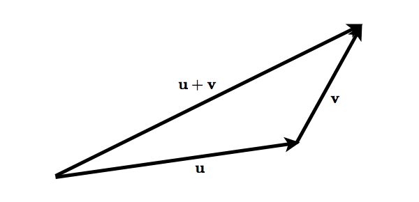 Figure 4: Illustrating the triangle inequality in 2-dimensional space
Defining a norm for a vector space allows us to characterize any given vector by a single, positive scalar value, i.e. the norm gives us an easy way of comparing vectors in the same space. The "trouble" with norms, though, is that there are so many of them and we need to choose one that's appropriate in the sense that it represents the entities of the problem we are trying to solve, and that the norm is computable at a tolerable cost.
The p-norm
The class of \(p\)-norms is a generalization of the Euclidean length of a vector \eqref{eq:euclidean_length_of_vector} and has many applications in mathematics, physics, and computer science. The \(p\)-norm is also known as the \(L^p\)-norm, and is for any real number \(p \ge 1\) defined by $$\begin{equation} \label{eq:p-norm_definition} \left\lVert \mathbf{v} \right\rVert _p = \left(\sum\limits_{i=1}^n \left\lvert v_i \right\rvert ^p \right) ^\frac{1}{p} \end{equation}$$ where \(\mathbf{v} \in \mathbb{R}^{n}\) and \(\left\lvert v_i \right\rvert\) is the absolute value of the \(i\)th element of the vector \(\mathbf{v}\). It can indeed be shown that \(\left\lVert \cdot \right\rVert _p\) defines a vector norm, but it's beyond the scope of these notes.
The \(L^1\)-norm
Setting \(p=1\) gives us the \(L^1\)-norm $$\begin{equation} \label{eq:1-norm_definition} \left\lVert \mathbf{v} \right\rVert _1 = \left\lvert v_1 \right\rvert + \left\lvert v_2 \right\rvert + \cdots + \left\lvert v_n \right\rvert \end{equation}$$ i.e. the \(L^1\)-norm for a given vector is the sum of the absolute values of all elements of the vector. The \(L^1\)-norm is also known as the taxicab norm since an analogy is offered by taxies driving in a grid street plan (like e.g. that of Manhattan) - such taxies should not measure distance in terms of the length of the straight line between their starting point and destination, but in terms of the rectilinear distance* * The rectilinear distance is defined as the distance between two points measured along axes at right angles. between the two points.
The \(L^2\)-norm
For \(p=2\) we have the \(L^2\)-norm - the well-known Euclidean norm that we saw in \eqref{eq:euclidean_length_of_vector} $$\begin{equation} \label{eq:2-norm_definition} \left\lVert \mathbf{v} \right\rVert _2 = \sqrt{\sum\limits_{i=1}^n v_i^2} = \sqrt{v_1^2 + v_2^2 + \cdots + v_n^2} \end{equation}$$ Combining this with \eqref{eq:inner_product_transpose_notation} we notice that the \(L^2\)-norm for a vector \(\mathbf{v}\) can be expressed in terms of the vectors inner product with itself $$\begin{equation} \label{eq:2-norm_expressed_by_inner_product} \left\lVert \mathbf{v} \right\rVert _2 = \sqrt{\mathbf{v}^\top \mathbf{v}} \end{equation}$$ The \(L^2\)-norm is probably the most commonly encountered vector norm, and is often referred to simply as the norm.
The \(L^\infty\)-norm
The special case where \(p = \infty\) is defined as $$\begin{equation} \label{eq:max-norm_definition} \left\lVert \mathbf{v} \right\rVert _\infty = \max_{1 \le i \le n} \left\lvert v_i \right\rvert \end{equation}$$ i.e. the \(L^\infty\)-norm gives you the absolute value of the vector element that has the largest absolute value of all the elements of the vector. Hence this vector norm is also known as the max-norm.
Example
The table below summarizes the vector norms discussed above (plus a couple more :-). Furthermore the values of the norms are given for the example row vector \(\mathbf{v} = \begin{bmatrix} 1 & 2 & 3 \end{bmatrix}\).
| Name | Symbol | Value for v |
|---|---|---|
| \(L^1\)-norm | \(\left\lVert \mathbf{v} \right\rVert _1\) | 6 |
| \(L^2\)-norm | \(\left\lVert \mathbf{v} \right\rVert _2\) | \(\sqrt{1^2 + 2^2 + 3^2} \sim 3.742\) |
| \(L^3\)-norm | \(\left\lVert \mathbf{v} \right\rVert _3\) | \(\left(1^3 + 2^3 + 3^3\right)^\frac{1}{3} \sim 3.302\) |
| \(L^4\)-norm | \(\left\lVert \mathbf{v} \right\rVert _4\) | \(\left(1^4 + 2^4 + 3^4\right)^\frac{1}{4} \sim 3.146\) |
| \(L^5\)-norm | \(\left\lVert \mathbf{v} \right\rVert _5\) | \(\left(1^5 + 2^5 + 3^5\right)^\frac{1}{5} \sim 3.077\) |
| \(L^\infty\)-norm | \(\left\lVert \mathbf{v} \right\rVert _\infty\) | 3 |
To gain a better intuition for the \(L^p\)-norms it might be helpful to consider how their unit circles are rendered in 2-dimensional space. A unit circle is centered at the origin of the coordinate system \((0, 0)\) and has a radius of \(1\), i.e. all points on the circumference have a distance of \(1\) from the origin. Under the Euclidean norm (the \(L^2\)-norm) this renders as the well-known "circular circle", but for the other norms the unit circle looks quite different.
The illustration of unit circles in various p-norms is courtesy of Wikimedia Commons and is distributed under a Creative Commons Attribution-ShareAlike license.
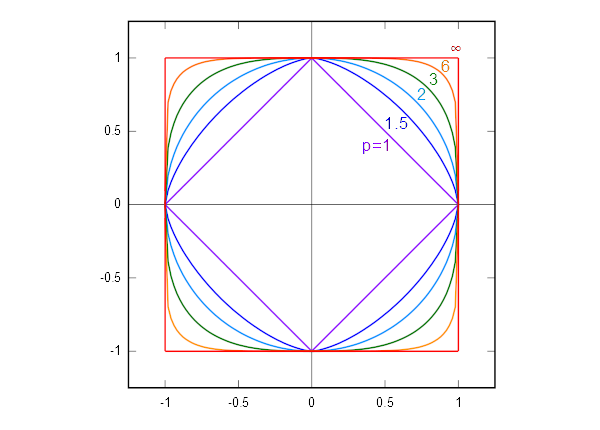 Figure 5: Unit circles in various p-norms
The formula for the unit circle in 2-dimensional \(L^1\)-norm geometry is \(\left\lvert x \right\rvert + \left\lvert y \right\rvert = 1\), i.e. the \(L^1\) unit circle is a square with sides oriented at 45° angles to the axes of the coordinate system. Similarly the unit circle in \(L^\infty\) geometry is also a square, but with sides parallel to the coordinate axes (i.e. the \(L^1\)-norm can be changed into the \(L^\infty\)-norm by a 45° rotation and a suitable scaling). This is illustrated in figure 5 above along with superelliptic unit circles in different p-norms.
In 3-dimensional space the unit ball for the \(L^1\)-norm is a octahedron, for the \(L^\infty\)-norm a cube, and for the \(L^2\)-norm the unit ball is the well-known sphere.
References
- [Boyd2018] Stephen Boyd & Lieven Vandenberghe, Introduction to Applied Linear Algebra - Vectors, Matrices, and Least Squares, Cambridge University Press,
- [IFEM2017] Introduction to Finite Element Methods, Linear Algebra: Vectors, University of Colorado at Boulder,
- [Lambers2010] Jim Lambers, Lecture 2 Notes (on Numerical Linear Algebra), The University of Southern Mississippi,