The building blocks of artificial neural networks are artificial neurons. These are modelled on their biological counterparts so we'll start out by having a brief (and extremely simplified) look at these. The aim is to gain a basic understanding of the essential information processing ability of real, biological neurons, while lightly skipping across most of the gory complexity of biological neural nets.
Biological neural nets
A typical biological neuron comprises
- dendrites, a tree-like structure that receives signals (i.e. information) from other neurons
- a cell body that processes the incoming information
- an axon that communicates information from the cell body to other neurons via synapses
The neuron SEM image is courtesy of Nicolas P. Rougier who made it available under a Creative Commons BY-SA 4.0 license. The image on the left is a color inverted version of the original which you can find here, showing amazing details.
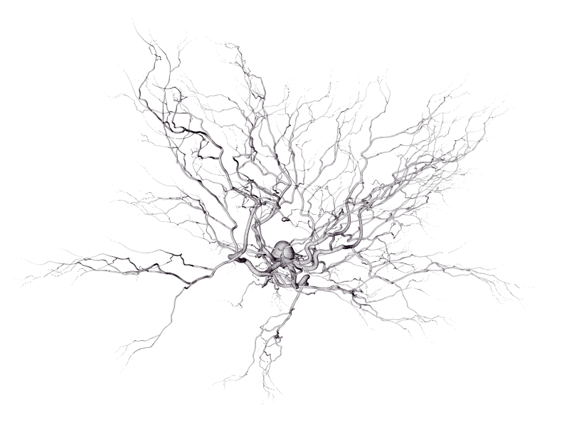 Figure 1: Scanning electron microscope (SEM) image of a biological neuron
A neuron receives incoming signals from its neighbors through its dendrites, where each of the terminal branches connect to another neuron (this connection is established via a synapse from the axon of the transmitting neuron). The amount of influence the signal has on the receiving neuron is decided by the synaptic weight (strength) of the connection between the firing and receiving neuron. The neuron combines the incoming signals and passes the result on to its axon. If the strength of the resulting signal is above a certain threshold, an outgoing signal will be passed on (fired) to other neurons via synaptic connections.
So in short a neuron exhibits the following behaviour:
- it receives weighted input from various other neurons
- these signals are combined and processed by the receiving neuron
- if the strength of the resulting signal is above a certain threshold, the neuron fires an output signal to neighboring neurons
In the following we'll use these ideas for modelling artificial neural networks. But as hinted by the above SEM image of a neuron, biological neural nets can grow extremely complex. It's estimated that the average human brain has about 100 billion (\(10^{11}\)) neurons with as many as 1,000 trillion (\(10^{15}\)) synaptic connections - a complexity that current artificial neural networks are not even beginning to be close to match!
The artificial neuron
A very simple model of a biological neural network could be represented by a weighted directed graph* featuring some additional capabilities. * A directed graph is a set of vertices - or nodes - connected by edges, where the edges have a direction associated with them.
In this model the artificial equivalent of a biological neuron is represented by a node in the graph. The edges of the graph correspond to synaptic connections, where the weight of an edge represents the amplification/dampening of the "signal" that's transmitted along that specific edge. Furthermore each node has the capability of deciding - based on the combined incoming weighed signals - what signal should be passed along its outgoing edges.
This "capability of deciding" is implemented by an activation function (sometimes also referred to as a transfer function) that takes the combined weighted input of the node - called the activation - and computes an output signal. I.e. the activation function can be said to model the behaviour of the axon of a biological neuron.
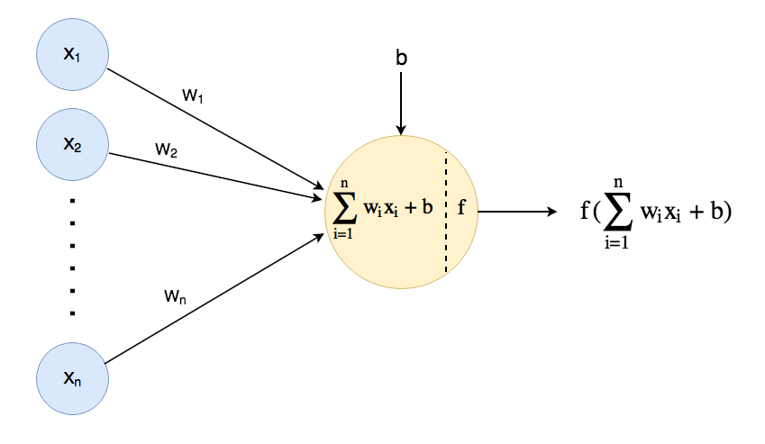 Figure 2: A generic activation function for an artificial neuron
The figure above shows \(n\) nodes, emitting values \(x_1\) to \(x_n\) respectively (corresponding to neurons sending signals along their axon). These values are amplified - or dampened - by the weights (\(w_1\) to \(w_n\)) of the edges transmitting the values (the biological analogy would in this case be synaptic weights influencing the signals between neurons). When the weighted output values are received by a node, they are added up along with a bias (the bias will be explained later). Finally an activation function is applied in order to decide the value to be propagated along outgoing edges to other nodes (this corresponds to a biological neuron combining incoming signals and "deciding" what output should be fired by its axon to connected neurons).
In summary, a generic activation function for an artificial neuron can be described as:
$$\begin{equation} \label{eq:activation_function} f(\sum\limits_{i=1}^n w_i x_i + b) \end{equation}$$Where \(x_1, ..,x_n\) are incoming values that are multiplied by their corresponding weights \(w_1\, ..,w_n\) before being added up. Then a bias, \(b\), is added to the result to obtain the activation of the node, and finally the activation function, \(f\), is applied.
The activation function, \(f\), can either be a binary function assuming discrete on/off values, perform a linear transformation to its input, or be a non-linear function†. † In a linear system, the output is always proportionally related to the input, i.e. small/large changes to the input always result in corresponding small/large changes to the output. Non-linear relations do not obey such a proportionality restraint. Below you'll find a brief introduction to some of the most widely used activation functions in artificial neural networks.
Examples of activation functions
Please note this list is currently a work in progress!
| Name | Description |
|---|---|
| The unit step function | 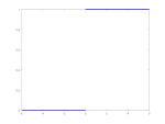 The unit step function is also known
as the Heaviside function. The function is defined as
\(u(x) = \begin{cases} 0 \text{, if } x \lt 0 \\ 1 \text{, if } x \ge 0 \end{cases}\)
and can be seen as a simple abstraction of a physical on/off switch.
The unit step function is also known
as the Heaviside function. The function is defined as
\(u(x) = \begin{cases} 0 \text{, if } x \lt 0 \\ 1 \text{, if } x \ge 0 \end{cases}\)
and can be seen as a simple abstraction of a physical on/off switch.
|
| The sigmoid function | 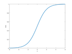 The sigmoid function, also
known as the logistic function, is a continuous, differentiable function defined as
\(\sigma(x) = \frac{1}{1 + e^{-x}}\).
The
derivative of the sigmoid function has a very convenient and beautiful form,
\(\frac{d\sigma(x)}{dx} = \sigma(x) \cdot (1 - \sigma(x))\), making it well suited for
back-propagation.
The sigmoid function, also
known as the logistic function, is a continuous, differentiable function defined as
\(\sigma(x) = \frac{1}{1 + e^{-x}}\).
The
derivative of the sigmoid function has a very convenient and beautiful form,
\(\frac{d\sigma(x)}{dx} = \sigma(x) \cdot (1 - \sigma(x))\), making it well suited for
back-propagation.
|